Simulation Verification and Validation Guide
“Trust Me, I’m an Engineer”
The goal of this article is to provide best practices for validating an application by comparing simulation results to experimental data. I will elaborately investigate one operating point and test representative properties for other working conditions and discuss how to ensure good results for one specific application. However, the concept can be used for any application and can therefore be used as a guide for other validation cases.
The Importance of Validation
You know it’s true: Simulation is only useful when it is reliable. From an engineering perspective, this means real world effects can be reproduced sufficiently. Validation helps to gain trust in the simulation method and the framework itself, but only for the validated property.
For example, Smoothed Particle Hydrodynamics (SPH) simulations of gearboxes have been proven to be a reliable tool to predict oil distribution1,2,3. One could call it validated. However, oil induced losses seem to be a lot harder to tackle in today’s SPH landscape.
Validation can be very specific, and it is essential to pick representative cases and directly validate the properties of interest. Looking only at simple academic cases is just not enough. Ideally, you have proof that your simulation software can predict all relevant effects in your geometry at all operating points. This can be a very tedious task, so we need a better system.
In this case, we validated a well-known test gearbox for a slow circumferential speed regarding aeration, velocity profile, and streamlines. If these aspects are in sufficient accordance with experimental measurements, we expect the oil distribution to be represented well. Churning losses are validated for mid-range rotation speeds. Because they depend on the oil distribution, we assume this is still represented well.
With the combination of both studies, the physical accuracy of the framework should become apparent, as discussed below. But let’s first find some reference data to compare with our simulations.
Reference data
The validation process of any simulation method is only feasible with high fidelity measurement data. A typical testing procedure requires accurately measuring the precise values of physical quantities of interest. Additionally, these results should be achieved repeatably under the same operating conditions.
Let’s talk gearbox: A no-load power loss test rig was designed at the Gear Research Centre (FZG) in Munich. The model is suited to investigate the oil dynamics and load independent losses in a simple dip lubricated gearbox. You can find the setup in several publications, offering various experimental data and simulation results obtained with different numerical schemes. It is the gearbox with most publicly accessible reference data. Especially the gear research departments at TU Munich, Chalmers University and their partners contributed a lot to our existing knowledge about the oil dynamics, the losses and numerical modelling of this gearbox.
The configuration type C used here features a box-shaped housing with one pair of spur gears. The bearings and sealings are well covered and can be decoupled from the oil dynamics in the gear domain. Some parts of the housing are transparent, which helps to gain visual insights and enables optical measurement techniques.
The oil level is constant for all conducted studies, featuring an immersion depth of 9 mm (2x the pinion module). Four multiphase simulations (air and oil are simulated at the same time) are presented here and validated against experimental data. The particle diameter is 1 mm for all simulations, which is sufficient to resolve the fluid pattern of interest. Circumferential speeds of 1.62, 10.5, 15.7 and 20 m/s are validated.
Visual Comparison
Of course, the most straightforward validation method is a visual comparison. It helps to estimate whether or not simulation results are plausible. Generally, this is only possible in cases where a phase interface can be observed.
However, it is often hard to get those insights in gearboxes. The housing is usually made of solid metal and closed in order to keep the oil from leaking. Most experimental setups use a transparent housing and good lighting to enable visual observations.
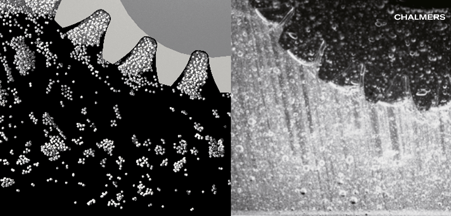
What reference data is available in our specific case? Ji et al.1 took laser induced fluorescence images to capture the bubbles in the test rig (Figure 3.). Already for a circumferential speed of 1.62 m/s, the teeth submerge air below the oil level, which partly causes the space in between the teeth to raise as bubbles move towards the surface. Both the size and distribution of these air bubbles can be used for the comparison.
The experimenters observed that the biggest bubbles fill almost the whole space between the gears and have an approximate diameter of 12 mm. Medium sized bubbles occur near the gear and have a diameter of 2 to 5 mm. Smaller bubbles are broadly spread.
Looking at the simulation, the space between the gears is comparably filled with air particles. It shows good accordance with the experiment. The medium sized bubbles are bigger and fewer than in the reference. Only some of them reach the bottom of the housing, which is also seen in the experiment. Few isolated particles indicate the smallest bubbles but can hardly be represented well in the simulation with the chosen resolution of 1 mm.
Overall, the captured air silhouette is in satisfying agreement.
Streamlines
To gain more insights into the flow within the lubricant, a Particle Image Velocimetry (PIV) evaluation was also conducted and published by Ji et al.1. For this technique, the fluid is seeded with small, spherical tracer particles that have approximately the same density as the fluid. Due to these characteristics, they are expected to follow the fluid pattern perfectly. Therefore, it is sufficient to observe only the particles as their behavior represents the flow. Usually, laser pulses are used to illuminate the particles in the plane to be evaluated. The scene is then photographed with the same high frequency of the laser pulses. The direction and speed of movement can be approximately reconstructed using correlation techniques on the particle positions on the images. More info on the method can be found here.
If you think that’s amazing but you don’t have a super expensive PIV system handy, I have a workaround: If you have access to MatLab, I can recommend the free application PIVLab that can be used to conduct the PIV evaluation technique for you recorded videos.
If the according measurement prerequisites are available to get the velocity vector field, streamlines are a great way to validate any Computational Fluid Dynamics (CFD) simulation. They represent the fluid behavior across the whole domain and therefore offer a good overall comparison.
The circumferential speed is once again at 1.62 m/s.
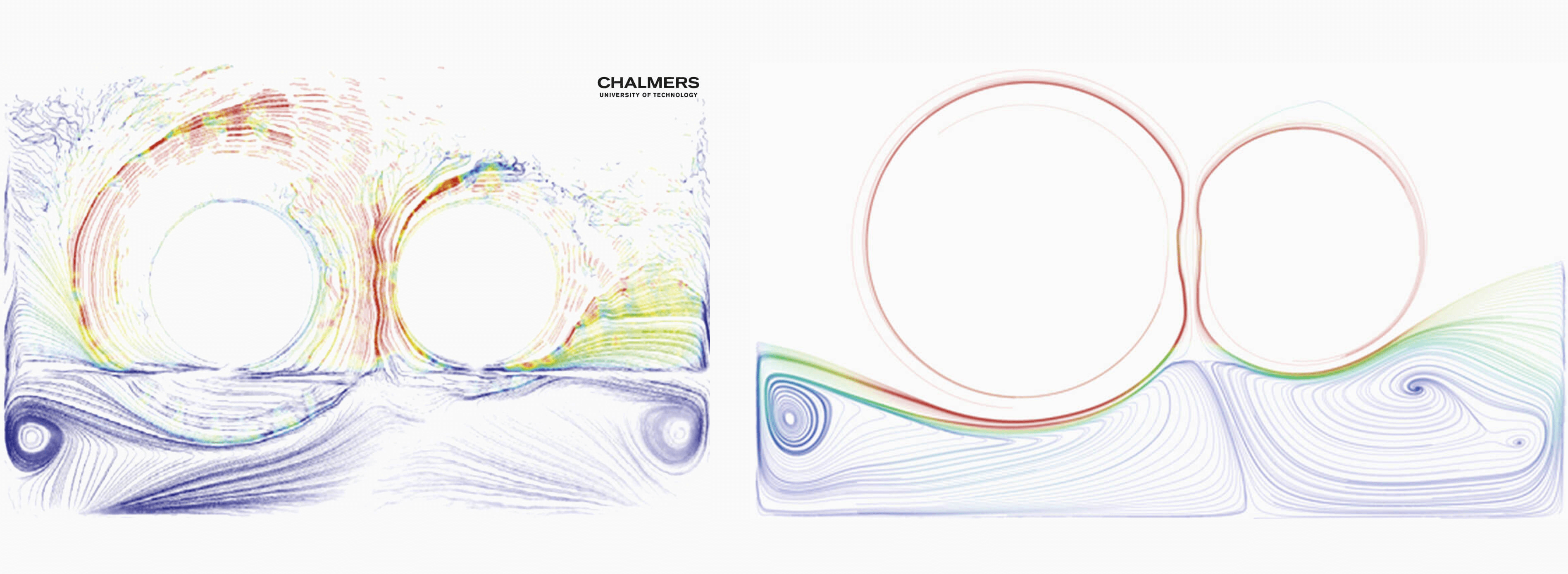
Left: PIV measurement close to the middle plane (Ji et al.)¹
Right: Streamlines in the SPH simulation in the middle plane
The respective PIV measurements for the present operation point are shown above. Here, two characteristic vortices can be seen in both corners of the gearbox. Their general shapes suggest similar origins: Both gears impose horizontal oil flows in the respective opposite direction which hit the wall and induces a stationary vortex. However, measurement errors are expected which are primarily related to the bubble formation in front of the measurement plane. They light up as bright as the tracer particles when hit by the laser. That’s why you see the oil level in front of the gears.
The streamline field of the SPH simulation shows reasonable results for the left-hand side of the oil flow. The right-hand side results show a distinct left-turning vortex which is not observed in the measurements. A similar derivation at this position was also found in the SPH simulations by Ji et al.1. However, if you look closer at the PIV image, you may see that the tail of the right vortex crosses though the position where we would expect it to be based on the simulation. Further, only the core of the missing vortex is missing, but the surrounding pathlines indicate its presence. We assume it’s an artifact of the bubble intake in the experiment, as previously discussed.
Velocity Profiles
A quantitative comparison of the fluid flow can be obtained by looking at the numerical values themselves. There is reference data for the absolute velocity profile below the wheel (the larger gear), obtained from the PIV measurements of Ji et al.1. For transient cases, you can measure the pressure e.g. over time at a certain point.
Here, the results of a multiphase simulation are presented as well as one simulation where the air particles were neglected (single-phase). This is a common simplification for SPH, as it reduces the computational effort, but it is not so easily possible in grid-based methods (see our article on SPH basics). Let’s look at the results and see if the negligibility of air is valid.
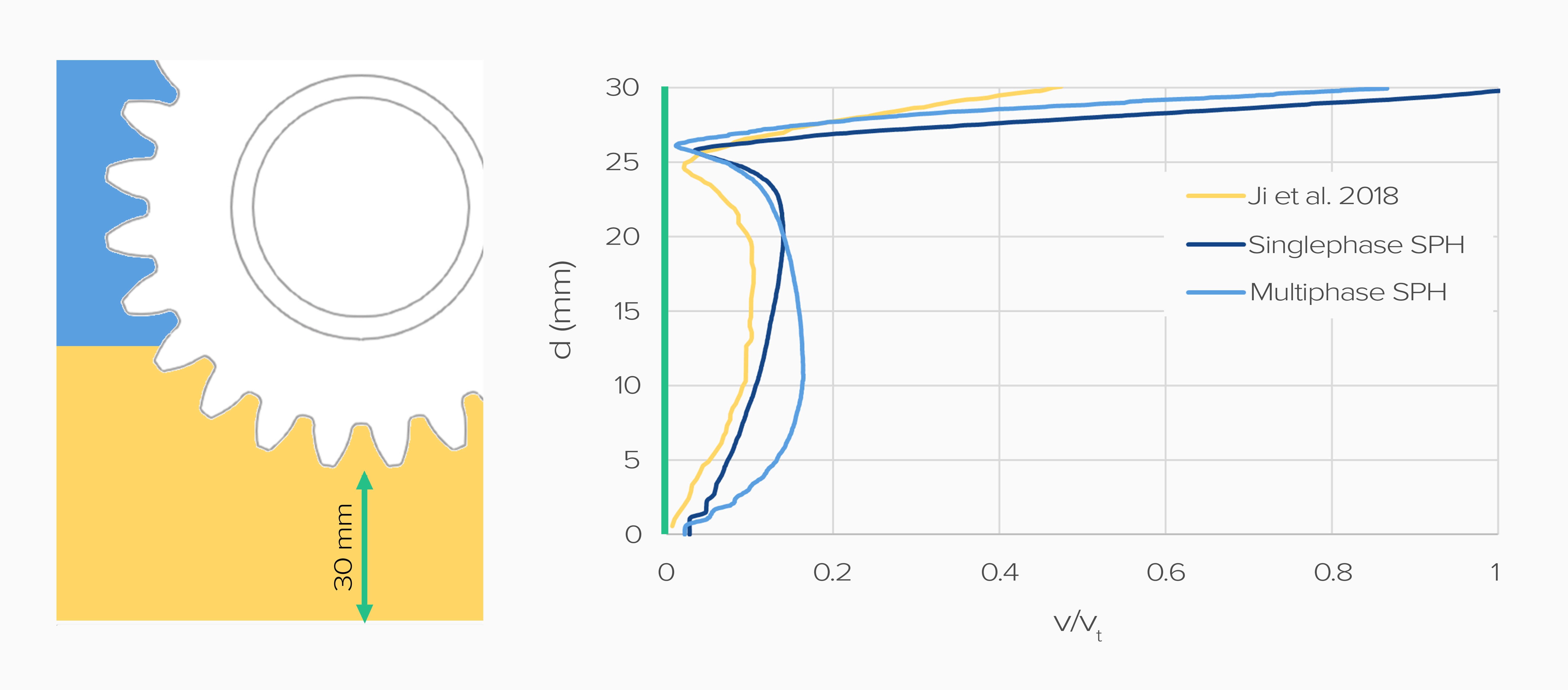
The y-axis in the plot above represents the distance from the bottom of the housing. The tip diameter of the wheel is at d = 0.031 m. It is surprising that the PIV measured curve is only at half of the expected circumferential speed at d = 0.03 m. This indicates a non-negligible PIV measurement error at the tip of the teeth. Although the turning point of the flow direction is well captured, the flow field underneath that point is less convex than the one detected by the simulation. Nevertheless, the results are in good agreement with the available data. Evidently, there is a difference between the single-phase and multiphase simulation. On the one hand, the results of the single-phase simulation show a similar velocity magnitude in the lower section. However, the qualitative shape of the multiphase curve matches more closely to the experimentally measured velocity profile. Don’t pin me down on the deviations here, we don’t know about the exact measurement error.
Churning Losses
Sustainability has become one of the biggest concerns of our time, especially for engineers (see our article about the Green Deal). Optimizing processes and minimizing losses are the name of the game. No-load losses can be a lever for high-efficiency transmissions. These losses can be interpreted as the effective power lost by moving fluid inside the gearbox. A more extensive guide on the different power losses in gearboxes and where they come from can be found in this article. Here you will find an in-depth explanation of how the losses can be measured in isolation.
From my experience, accurate churning loss prediction requires:
- A good approximation of the real geometry
- Sufficient representation of the movement and distribution of the lubricant
- Accurate pressure and viscosity induced forces
Therefore, they are an interesting value to validate because they are highly integrated. If the churning losses are in good agreement for various operating points, all properties above can be expected to be fulfilled. That means we can look solely at these points for the rest of the study.
Finding a highly integrated property like this is the key to efficiently validating an application for all operating points. But remember: It should also be easy to measure.
The reference measurements are taken from Liu et al.4, because they cover data for a broad range of circumferential speeds (10.5, 15.7 and 20 m/s). For lower speeds, the losses are smaller and harder to measure precisely. Higher speeds (more than 25 m/s) lead to very violent flow, often inducing foaming in oil and therefore a complex transition of material properties during the simulation. We would not expect to get very accurate results at that speed and reference data is not available anyway.
Figure 6: Rendering of the oil surface at the beginning of the simulation
Our measured churning power losses match the experiment and references very well. The SPH results are comparable to those of the Finite Volume (FV) simulation (to learn more about FV and other types of CFD, check out our article, CFD Methods). Not only is the tendency covered, but the time-averaged losses for all operating points are within the range observed in the experiments.

Conclusion
We hope this explanation has given you a good understanding of the importance of application validation and how it works. Let us know if you have any questions or want more information on any of the topics mentioned above by leaving a comment below.
Do you want to see more gearbox content? In one of our next articles, we will expand upon the work done with this gearbox and explore at the influence of different parameters. What is the role of surface tension at different circumferential speeds? How are the results affected by scaling the gears, which is common practice with grid-based methods?
If you don’t want to miss any articles, make sure to subscribe to our newsletter and follow us on LinkedIn!
1 Z. Ji, M. Stanic, E. A. Hartono and V. Chernoray, “Numerical simulations of oil flow inside a gearbox by Smoothed Particle Hydrodynamics (SPH) method”, Tribology International, Vol 127, pp. 47-58, 2018.
https://doi.org/10.1016/j.triboint.2018.05.034
2 M.C. Keller, S. Braun, L. Wieth, et al., “Numerical Modeling of Oil-Jet Lubrication for Spur Gears using Smoothed Particle Hydrodynamics”, Proceedings of the 11th International SPHERIC Workshop, Munich, June 13-16, 2016. 69-76. 2016.
https://doi.org/10.5445/IR/1000063565
3 H. Liu, G. Arfaoui, M. Stanic, et al., “Numerical modelling of oil distribution and churning gear power losses of gearboxes by smoothed particle hydrodynamics”. Proceedings of the Institution of Mechanical Engineers, Part J: Journal of Engineering Tribology. 2018.
https://doi.org/10.1177/1350650118760626
4 H. Liu, T. Jurkschat, T. Lohner, K. Stahl, “Detailed Investigations on the Oil Flow in Dip-Lubricated Gearboxes by the Finite Volume CFD Method”, Lubricants, 6. 47, 2018.
https://doi.org/10.3390/lubricants6020047